Approach
AJP Engineering provides high-quality optimized exchanger profile analysis consulting services. Our approach is presented below.
Heat Transfer
Heat exchangers cannot be characterized by a single design. However, the one characteristic that is common to most exchangers is the transfer of heat from a hot fluid to a cold fluid. For shell and tube heat exchangers, the fluids are separated by a solid boundary. A temperature difference is the driving force by which heat is transferred. Typically, it is up to the process engineer to design or specify heat-transfer equipment that meets certain process design requirements and to recommend methods that reduce heat losses in the operating plant.
The basic heat transfer equation is specified as follows:

Q = U * A * LMTD
where
Q ==> Total Exchanger Duty Rate [BTU/hr]
U ==> Overall Heat Transfer Coefficient [BTU/hr - sq ft - deg F]
A ==> Exchanger Surface Area [ sq ft]
The logarithmic-mean temperature driving force, LMTD, is
LMTD = [ΔT2 - ΔT1] / [ln(ΔT2 / ΔT1)]
ΔT1 & ΔT2 are the temperature driving forces at the exchanger terminals.
Multi-pass exchangers have a logarithmic-mean temperature difference that lies somewhere between true countercurrent and true concurrent. To correct this situation, a correction factor F is applied to the “true countercurrent logarithmic-mean temperature difference”. For true countercurrent flow, F = 1, and as more concurrent flow is introduced, this factor is reduced. The corrected logarithmic-mean temperature (CLMTD) is equal to the (counter LMTD) multiplied by the correction factor F.
The modified basic heat transfer equation is now:
Q = U * A * CLMTD
The Overall Weighted LMTD (OWL) method addresses the “enthalpy is linear function of temperature” assumption associated with the basic heat transfer equation. For varying specific heats or the contribution of either latent heat or heat of reaction, the enthalpy-temperature relationship is non-linear. This behavior is prevalent with exchangers in two-phase service. The introduction of enthalpy-temperature non-linearity invalidates the standard LMTD calculations. To overcome this limitation AJP Engineering employs the OWL method.
Overall Weighted LMTD (OWL) Method
Heat Release Curve
At the heart of the Overall Weighted LMTD (OWL) method is the heat release curve.
The OWL design method requires the use of two (hot and cold side fluid) duty-temperature curves. The following figure presents an example Temperature-Enthalpy Curve generated by the AJP Engineering proprietary C# application – AJP Exchanger 4.
The OWL design method requires the use of two (hot and cold side fluid) duty-temperature curves. The following figure presents an example Temperature-Enthalpy Curve generated by the AJP Engineering proprietary C# application – AJP Exchanger 4.
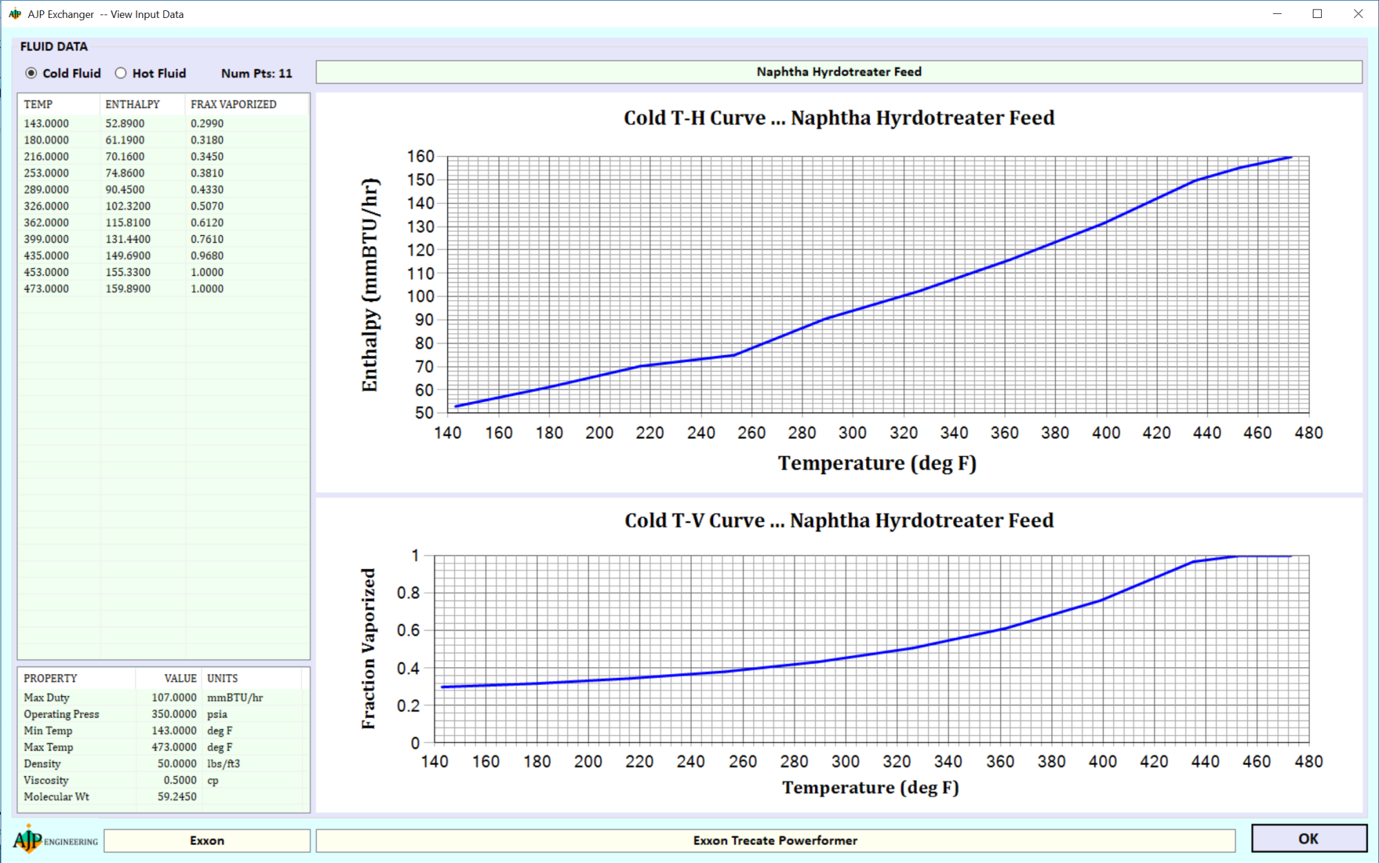
The hot and cold fluid enthalpies at the process conditions are transformed into exchanger duties. The duties are calculated relative to the input hot terminal and output cold terminal enthalpies for the hot and cold fluids respectively. The plot of duty versus temperature is defined as the heat release curve, where duty and temperature are the independent and dependent variables respectively (i.e., temperature = f(duty) ).
The following figure shows an example Heat Release Curve generated by the AJP Engineering proprietary C# application – AJP Exchanger 4.
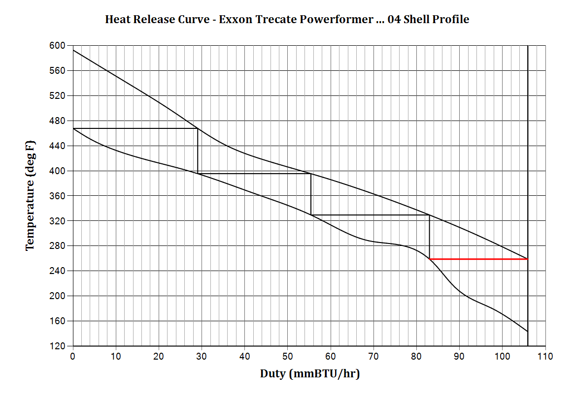
The OWL Method consists of breaking the heat release curve into linearly approximated zones. For each zone the LMTD, F, and CLMTD values are calculated. Overall LMTD, F, and CLMTD values are calculated on a duty-weighted average basis.
Optimized Exchanger Shell Profile
In order to determine the minimum number of exchanger shells, as well as the actual shell partition-profiles, equal outlet temperatures are assumed. Graphically this is represented by horizontal tie-lines on the heat release curve. Each horizontal tie-line is considered a shell. Note that under the equal outlet conditions for the shell the correction factor is optimized (F factors approximately 0.80). Also note that the last shell in the exchanger series may, or may not, be at equal outlet conditions. This shell is used to determine if further optimization is required.
Each exchanger shell obtained from the “equal outlet tie-line step-off” method is analyzed to determine if the heat release curves, over the shell range, are “linear”. For the graphical method this is accomplished by “eye-balling” the curves.
The AJP Engineering proprietary application utilizes cubic spline technology to represent the curves; analogous to using a French curve versus a straight edge ruler. Numerical Analysts recognize the value in using cubic splines to represent curve inflections; curve inflection representation is important for exchangers in two-phase service. AJP Engineering utilizes proprietary spline algorithms to achieve optimum curve representation.
In addition, AJP Engineering utilizes proprietary numerical analysis root-finding algorithms to perform the horizontal step-off procedure for shelling and zoning the exchangers.
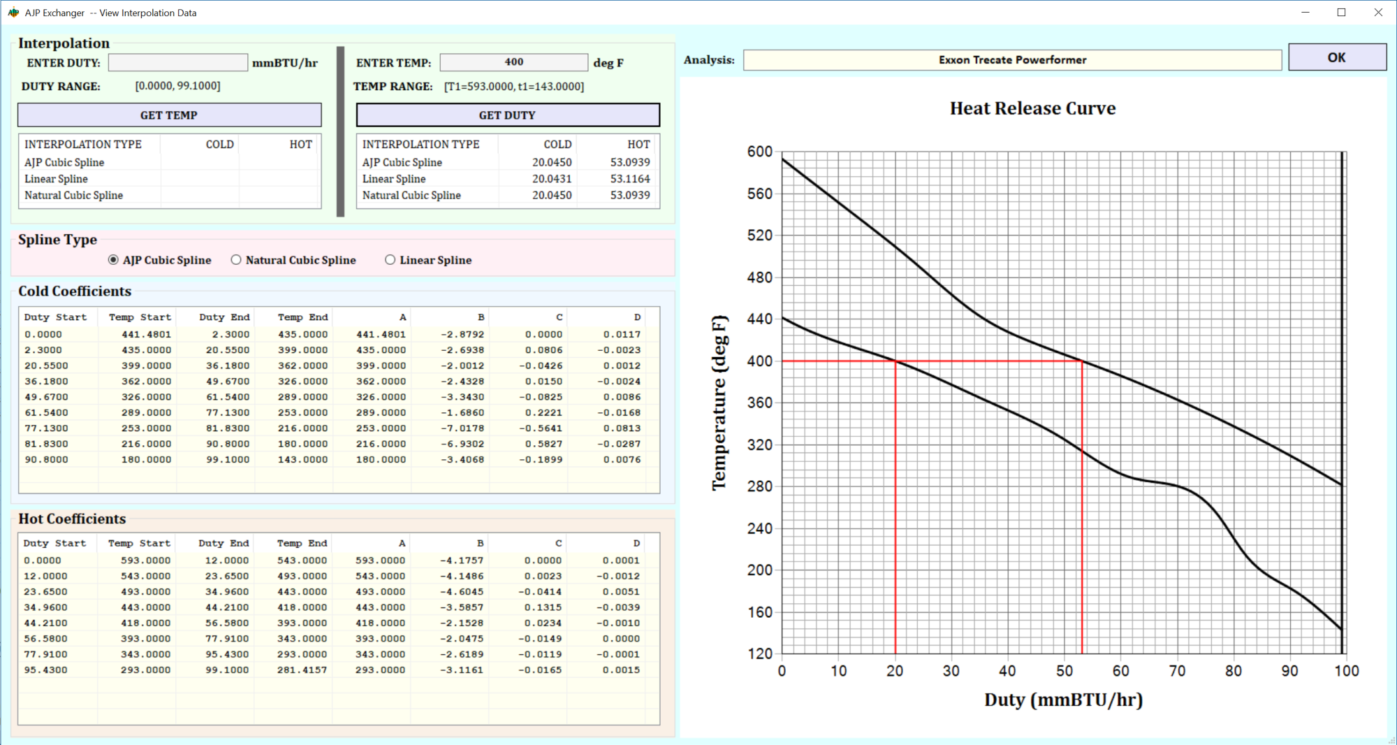
The following is an Interpolation form screen shot from the AJP Engineering proprietary C# application – AJP Exchanger 4.
Each exchanger shell obtained from the “equal outlet tie-line step-off” method is analyzed to determine if the heat release curves, over the shell range, are “linear”. For the graphical method this is accomplished by “eye-balling” the curves.
The AJP Engineering proprietary application utilizes cubic spline technology to represent the curves; analogous to using a French curve versus a straight edge ruler. Numerical Analysts recognize the value in using cubic splines to represent curve inflections; curve inflection representation is important for exchangers in two-phase service. AJP Engineering utilizes proprietary spline algorithms to achieve optimum curve representation.
In addition, AJP Engineering utilizes proprietary numerical analysis root-finding algorithms to perform the horizontal step-off procedure for shelling and zoning the exchangers.
The following is an Interpolation form screen shot from the AJP Engineering proprietary C# application – AJP Exchanger 4.